Please weigh in on photon noise

See the link posted here: www.dpreview.com/forums/thread/4710831?page=3#forum-post-67026232. The wave packet theory is in the past, it seems.

Interesting post, I can't comment on wave/particle duality because I understand the issue has not been satisfactorily resolved yet. But with regards to Purcell's comment above, perhaps they are not Newtonian physics analogies, rather observations that can be explained statistically at pixel scale thanks to Planck/Einstein and others.

For instance if one were to assume that the raindrops falling in one bucket arrived at a certain rate but with random timing without collisions, they would arrive with the observed Poisson distribution. Just like photons from a source landing on a pixel's photodiode. And we can actually measure the relative counts.

Jack

Jack's post above made me take another look at this post of AShortUserName. There is so much misinformation even in that paragraph, I do not even know where to start. "Light waves can interact with each other" - not in the linear model mentioned later. "When groups of light waves are in superposition (the definition of a wave packet)" : no, this is not a definition of a wave packet, you are thinking of a superposition of wave packets, as Tao says. "They interact with each other": actually, a superposition means linearity (a sum) which is on the opposite side of interaction. "The Schrödinger equation applies [3]": it does not, it is the QED for photons but even if we forget that, the (linear) Schrödinger equation excludes interaction, and we do have a superposition. "The result is an amplitude (i.e. non-classical)  probability distribution (Purcell's "abnormal density fluctuations") in photoelectron production": this is not even wrong, it just does not mean anything.

A stimulating video. However, he loses me when he says

On the contrary, the spatial/time probability of detecting a photon is indeed quantized, as we have been able to observe for quite some time once we got clean detectors, see for instance recently Eric Fossum's QIS work:.

As he explains, the Gaussian looking shapes around each peak are the result of the convolution of the detector's read noise with impulses representing the discrete Poisson distribution of actual detected counts. As detector read noise gets smaller and smaller, the resulting probability distribution tends to the discrete Poisson probability mass function.

So if the resulting probability (light*detection) is quantized with a Poisson distribution, what can we say about the field from the source?

We know from an earlier post that Poisson*Binomial = Poisson, therefore the field being quantized would match observation.

What class of continuous field probability distributions times Binomial detection would result in a Poisson distribution out?

Jack

I tried to keep it simple, let me know if you have any suggestions for improvement:

www.strollswithmydog.com/photons-poisson-shot-noise/

Jack

I gave it a quick look, and have two major remarks (and a few more minor ones, like you use the term variance a bit too loosely, while it should be reserved for the square of the standard deviation):

When you add the two standard deviations in quadratures, in other words, you add the two variances, which property do you use? If you have two independent noises added to each other, their variances add, indeed. This is not the case here, however. First, the standard view of noise is to have zero mean, and none of those two random variables has zero mean. This is not a big problem because one can adjust for it easily but it has to be done. Most importantly, you are not adding binomial noise to Poisson one. It is not like you have 100 photons in average, +/-10, and you randomize them additionally by adding binomial fluctuations with variance 100QE(1-QE) (and mean 100QE?). The effect of QE<1 is not additive noise; it is a composition of random variables in my understanding (like in conditional probability). In the end, your calculations get the right answer, and there might be a way to explain why that I do not see now, but the way it is presented is not right.

Also, you get a standard deviation corresponding to a Poisson process with mean s*QE. That, by itself, does not mean that the process is Poisson. It is just a happy coincidence. To show that the new process is Poisson, you need to verify its defining properties, and you actually did so in your posts here earlier. Or do the calculation I did.

Thanks JACS, much appreciated, I'll put some thought into how to explain it better without complicating things too much.

Jack

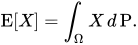
No, it does not mean that. In our case, it is the mean of the process creating it with respect to the probability measure. This is reflected by the formula defining is a integral of x times dP(x), where the latter is the probability measure. We have to give it some catchy name, and we call it "expected value." We could have called it a "cow" but it would have been less intuitive.

Again, there is the expected value of the process and the mean of finitely many samples. Those are different animals. The latter converges to the former with infinitely many samples but for every finite number, it is only "close."

EDIT: Let me give an example: You roll a die, once at a time. The process gives you 6 possible outcomes with probability 1/6 each. The expected value is 3.5, which ironically never happens. It is the weighted average of all outcomes with weight 1/6, which happens to be the arithmetic mean as well. Now, you roll it 10 times. You are not going to get a mean 3.5 most likely. Roll it 100 times. You will get closer with high probability, roughly speaking, etc. The expected value of the process is still 3.5.

In another thread on this forum, I made a coarse demonstration of the random arrival times, but used block code instead of a graphic, so I was stuck with low resolution, which gives a general idea, but with unrealistic spacing that is more consistent than the real thing:

             TIME->
Ideal:  0     1     2     3     4     5     6     7     8     9
Real-A: 0 1     2  3  4           5            6 7          8
Real-B: 0   1    2 3             4     5        6    7  8 9  10

Running some actual code in Processing, though, we get much more variety in spacing, which, in a car model, might indicate a lot of "tailgating":

  size(500,200);
  for(int x=0;x<width;x++)
  {
    if(random(1)<0.03) line(x,0,x,height); 
  }

It is always the mean with respect to the probability measure, just by definition.

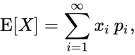
For a Poisson distribution, the probability to have value k is where λ is the expected value. That is the measure at the outcome X=k. The expected value is the mean with respect to that measure, i.e., the weighted average: Σ k. exp(-lambda)λ^k/k!, the summation is over k=0,1,... It is very easy to show that this equals λ, indeed. So this is the expectation of the process. When you start sampling it, we get a mean of the samples close to it with the number of samples going to infinity. Now, this is a conventional mean.

Perhaps one would expect a sequence of values from a sequence of samples ... 😉
...

Here: en.wikipedia.org/wiki/Expected_value#Arbitrary_real-valued_random_variables

As they say there: Despite the newly abstract situation, this definition is extremely similar in nature to the very simplest definition of expected values, given above, as certain weighted averages. This is because, in measure theory, the value of the Lebesgue integral of X is defined via weighted averages of approximations of X which take on finitely many values. Moreover, if given a random variable with finitely or countably many possible values, the Lebesgue theory of expectation is identical with the summation formulas given above. However, the Lebesgue theory clarifies the scope of the theory of probability density functions.

In particular, here: en.wikipedia.org/wiki/Expected_value#Random_variables_with_countably_many_outcomes

Informally, the expectation of a random variable with a countable set of possible outcomes is defined analogously as the weighted average of all possible outcomes, where the weights are given by the probabilities of realizing each given value.

See also the second paragraph on p.386 here: link.springer.com/content/pdf/10.1007/978-3-030-33143-6_12.pdf

Good one John. This is what I came up with for photons in 2D (it's a GIF, so click on it to see the simulation)

And this is the histogram for a constant mean rate of 5.2 random events per unit of time or space

generated with this self evident code in Matlab: 104,000 events over 20,000 slots

Full code for the figures above in the notes of the relative article.

Jack

I am not very good at reading pseudo codes or even actual ones. What is the code doing here? Throwing away integers in random, and then you count how many are left in an interval of length n, like in [1, n], [n+1,2n], etc.? If so, this is not Poisson.

It looks like he's doing 500 Bernoulli trials with p=0.03. So it's an approximation to Poisson. Seems good enough.

Maybe you would prefer something like:

double last_arrival_time = 0.0;
for( int i = 0; i < n_arrivals; ++i )
{
   double wait = -log( 1.0 - random(1) ) / lambda;     // Exponentially distributed, parameter lambda
   last_arrival_time = last_arrival_time + wait;
   arrival_time[i] = last_arrival_time;
}
// At this point, last_arrival_time has distribution Erlang(n_arrivals, lambda)